Qiskit Version 1.0 Crash Course: How to Build a Quantum Circuit

How Do You Build a Quantum Circuit?

For quantum computer scientists, one of the most crucial steps in their journey into quantum lies in their first quantum circuit. The most commonly used, entry-level language for coding quantum circuits and algorithms is the Qiskit language, developed by IBM.

Over the last year, the IBM’s Qiskit has undergone a number of changes, emerging on the other end as Qiskit version 1.0. These changes introduce a series of moved and, more crucially, a different way of running your quantum circuits.

However, for beginners, the documentation for these programs can be scary, so we will create your quantum “Hello World” equivalent program below and answer the question: how do you run a quantum circuit?

Setting Up Your Account on a Cloud Server

To run your code on a real quantum computer, set up an account with the IBM Quantum Platform which, as of the time of writing, should be free to access (with limited compute time on a quantum computer).

To create a Quantum Platform account, visit https://quantum.ibm.com and select “Create Account” under the “Open Plan.” This plan offers up to 10 minutes of runtime on quantum systems each month — more than sufficient for a series of introductory quantum programs.

The code we have below was tested on Google Colab for ease of use and sharing. For instructions and more information on Google Colab, here is a good article to get you started. Regardless, you are more welcome to run this on your local computer or another platform.

Preparing Your Environment

Your “environment” refers to the space you are running your program in — this can include any packages (“tools” to help out with your program) that you install, specified language versions, and so on.

In the current day and age, you unfortunately do not have access to a personal quantum computer. Instead, you will need to connect to one of the major quantum computers around the world hosted by IBM.

To do so, let us first install some packages that will help us with our quantum journey. This section may take a moment to run.

If you get an error that says, “ERROR: pip’s dependency resolver does not currently take into account all the packages that are installed,” do not worry, the specified packages should not interfere in our sample circuit below.

%pip install qiskit[visualization]==1.0.2 # installs Qiskit version 1.0.2

# install other helper packages
%pip install qiskit_aer
%pip install qiskit_ibm_runtime
%pip install matplotlib
%pip install pylatexenc
%pip install qiskit-transpiler-service

In order to keep track of tasks that are submitted to be run, the IBM Quantum Platform takes in what is known as your API token to access your account. Do not under any circumstance share this key publicly or with untrusted parties as it will give anyone with access to it free access to the operations on your account.

To retrieve your quantum API token, log into your IBM Quantum account. This will take your to your IBM Quantum Dashboard, which looks like the following.

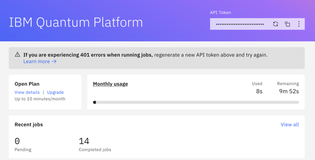
In the top right of the dashboard, look for the section titled, “API Token.” Click on the copy button to copy the entirety of the API token. In the case your API token is accidentally leaked, do not worry — click on the refresh button to generate a new token.

Return to your code and run the following line. Be sure to replace the words “Your API Token Here” with the API token you copied for your account. Do not leave a space between the “=” sign and the characters in your token.

# replace Your API Token with your own API token.
%set_env QXToken=Your API Token
# Make sure there are no whitespace characters between the = and your token. 
# For example, QXToken=123 is valid, but QXToken= 123 is not.

# import the packages installed to your environment
from qiskit import QuantumCircuit
from qiskit.primitives import StatevectorSampler
from qiskit.transpiler.preset_passmanagers import generate_preset_pass_manager
from qiskit.visualization import plot_histogram
from qiskit_ibm_runtime.fake_provider import FakeSherbrooke
from qiskit.quantum_info import SparsePauliOp
from qiskit_ibm_runtime import EstimatorV2 as Estimator
from qiskit_aer import AerSimulator
import matplotlib.pyplot as plt

import numpy as np

Setting Up Your Circuit

Once you have connected your quantum account, let’s try to build your first circuit! Before running any dramatic quantum algorithms, let’s try to create a superposition of two qubits. For a rundown on what superposition and other key concepts in quantum computing are, check out this blog post.

To do so, we will try to build one of the four possible Bell States, namely

If you are uncertain of what this means, don’t worry! The values in the |> represent the values of the quantum bits (qubits). For example, |10> means that the first qubit has the value 1 and the second qubit has value 0. Similarly, |00> means that the first and second qubits both have value 0. Furthermore, squaring the coefficient of corresponding to each of the |> indicates our probability of measuring the system to have those values.

With this in mind, the above equation means that for our two qubits, we have a 1/2 probability of measuring both qubits as 0 and a 1/2 probability of measuring both qubits as 1. Observe that the total system, named phi+, can possibly be two possible states: either |00> or |11>. This indicates that the quantum system is in what is known as a superposition. We create this Bell State below.

If you are unfamiliar with quantum gates, that is okay! For the time being, aim to understand what each section of code approximately does.

# create an object that is of type QuantumCircuit with two qubits.
circuit = QuantumCircuit(2)

# We will add gates ("operations") to this object below, much like how you may add a series of machines to assembly lines.
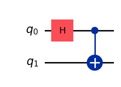
circuit.h(0) # add a Hadamard gate to the zeroth qubit (labelling the qubits starts at 0 and goes to 1, 2, ...)
circuit.cx(0, 1) # add a CNOT controlled by the zeroth qubit and applied to the first qubit

# visualize the circuit below
circuit.draw('mpl')

Expected output:

Using the State Vector Sampler

The Bell State

is what is known as a state vector — the type of notation used leans on key concepts of linear algebra. The state vector sampler in Qiskit derives its name from this concept. The idea is as follows:

• Quantum computers are probabilistic in nature. That is, when your qubits are in a superposition (as those in the Bell States are), there is a non-zero probability (and also not 100% chance) associated with measuring the system to be in some state.
• To illustrate this probability, the state vector sampler “samples” the circuit a large number of times and measures the results. That is, the circuit is run, the qubits measured, and the results recorded.
• The distribution of these results should approximately correspond to the theoretical state vector. This is like how flipping a coin once doesn’t give much information about the probability of getting heads or tails on the coin. However, flipping a coin 1000 times has an expected distribution of about 500 heads and 500 tails, which shows that we have an expected $\frac{1}{2}$ probability of measuring each state of the coin.

We will use the StatevectorSampler to accomplish this series of samples.

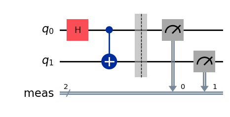
# indicate that you want your quantum circuit to measure all qubits at the end
circuit.measure_all()
# illustrate the circuit with the measurements
circuit.draw('mpl')

Expected Output:

# create an instance of the Qiskit StatevectorSampler
sampler = StatevectorSampler()

# run the job on the StatevectorSampler, passing in the circuit. There will be 256 samples taken.
job_sampler = sampler.run([(circuit)], shots=256)

# get the results from the sampler
result_sampler = job_sampler.result()

# to get a dictionary of data mapping {state : number of samples}, we use get_counts()
counts = result_sampler[0].data.meas.get_counts()
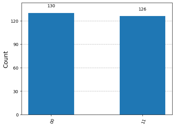
print(counts)

Example Expected Output: {’00’: 130, ’11’: 126}

# we can plot these counts to show the distribution of results
plot_histogram(counts)

Expected output (exact counts may differ):

Transpiling the Circuit

To run the circuit on a quantum computer, we must make sure that it fits the architecture of said quantum computer.

To do so, we first select a backend (with some architecture) to arrange our circuit around. In this case, we are going to base our transpiled circuit on the fake backend FakeSherbrooke(). To view all of the options for fake backends, feel free to review the documentation from IBM on fake providers.

What does transpiling a circuit mean?

This topic is worth an entire blog post of its own — the description provided here is far from sufficient in defining what “transpiling” a circuit can imply.

The Qiskit transpiler takes in a circuit and, through a series of steps (called passes), will alter the circuit so that it is optimized and fit to the actual arrangement of qubits and set of possible gates on a quantum computer.

At a low level, quantum computers have a small set of gates that they can use to recreate all of the different options we — as end users — can use — such as the simple X or Y rotations, or the CNOT gate. For example, a Toffoli gate (run on three qubits) is in fact made up of five two-qubit quantum gates. As such, the transpiler will first decompose the more complex gates in the circuit into gates that are runnable on the quantum computer.

From there, each of the qubits used in the circuit are matched with a physical qubit on the quantum computer. While this may seem simple at first, quantum computer architectures are not as simple as completely interconnected bits, so this takes some fanagling. SWAP gates may be inserted in the initial circuit to ensure connectivity. From there, the gates in the circuit may be “translated” into the target backend’s basis set (which may be seen as the “directions of measurement” when measuring the bits).

However, deomposing the circuit, inserting SWAP gates, and making these changes can dramatically increase how many gates — or operations — are being run. As such, the transpiler will try to optimize the circuit. This can include — but is not limited to — actions such as reducing the depth of the circuit (how many “layers” of operations are applied) and switching out gates and cancelling inverses.

Once this final circuit has been reached, some minor changes are made to prevent idle qubits (which risk decoherence), and the circuit has been rearranged to be run.

Additional technical details are accessible here.

While a custom transpiler and optimizer may be built, we use a preset pass manager to build our transpiler.

# redefine the circuit
# create an object that is of type QuantumCircuit with two qubits.
circuit = QuantumCircuit(2)

# apply quantum gates to construct the Bell State
circuit.h(0)
circuit.cx(0, 1)

# set the parameters for generating the transpiler
backend = FakeSherbrooke()
optimization_level = 1 # for a description of optimization levels, visit: https://docs.quantum.ibm.com/api/qiskit/transpiler#optimization-stage

# generate the pass manager with these parameters
pass_manager = generate_preset_pass_manager(backend=backend, optimization_level=optimization_level)

# transpile the circuit
transpiled_circuit = pass_manager.run(circuit)

# visualize the transpiled circuit
transpiled_circuit.draw('mpl', idle_wires=False,)

Expected output:

This transpiled circuit is now prepared to be run.

Running a Circuit

In this tutorial, we will select to execute the circuit using an estimator, which estimates approximately how many show will fit a given set of values.

We will use the Qiskit Aer simulator as our backend, with documentation linked here.

To do so, we define the range of data that can possibly be outputed. This is saved in the data = ['IZ', 'IX', 'ZI', 'XI', 'ZZ', 'XX'] line. The I corresponds to applying an identity gate to the qubit, the Z corresponds to applying the Z gate to the qubit (a rotation of pi around the Z-axis), and similarly for the X gate.

# Z operator on 0, Z operator on 1
ZZ = SparsePauliOp('ZZ')
# Z operator on 0, I operator on 1
ZI = SparsePauliOp('ZI')
IX = SparsePauliOp('IX')
XI = SparsePauliOp('XI')
IZ = SparsePauliOp('IZ')
XX = SparsePauliOp('XX')

observables = [
    SparsePauliOp('IZ'),
    SparsePauliOp('IX'),
    SparsePauliOp('ZI'),
    SparsePauliOp('XI'),
    SparsePauliOp('ZZ'),
    SparsePauliOp('XX')
]

data = ['IZ', 'IX', 'ZI', 'XI', 'ZZ', 'XX']

# set up the Estimator to execute the circuit
# set the Aer Simulator object as the backend.
estimator = Estimator(backend=AerSimulator())

job = estimator.run(pubs=[(circuit, observables)])

# we can then get the set of results as follows
results = job.result()[0].data.evs

# to visualize the results
graph = plt.plot(data, results, '-o')

# label each axis
plt.xlabel('Observables')
plt.ylabel('Values')

plt.show()

Expected Output:

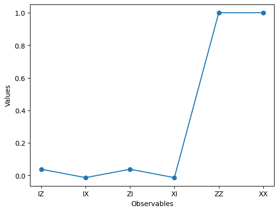
Observe that the values of ZZ and XX are close to 1 — the higher the value, the more likely they are to be measured and be outputted as a result. ZZ corresponds to |00> and XX corresponds to |11>.

Conclusion

With that, this concludes the tutorial — we discussed creating a basic quantum circuis, sampling the state vector of the circuit, and using an estimator to run the circuit on a simulator and obtain results.

There are plenty of alternative implementations — such as using a Hamiltonian on optimization problems or custom building transpilers — that are worthy of attention. Nonetheless, congratulations on taking a step deeper into the world of quantum computing!