In this tutorial, we will build a quantum machine learning algorithm that classifies and recognizes handwritten digits(whether a digit is 0 or 1) present in the MNIST dataset. We will make use of several dimensional reduction techniques, perform classical pre-processing and initialize our own quantum feature maps.
The following diagram gives a brief overview of the Variational Quantum Classifier protocol.
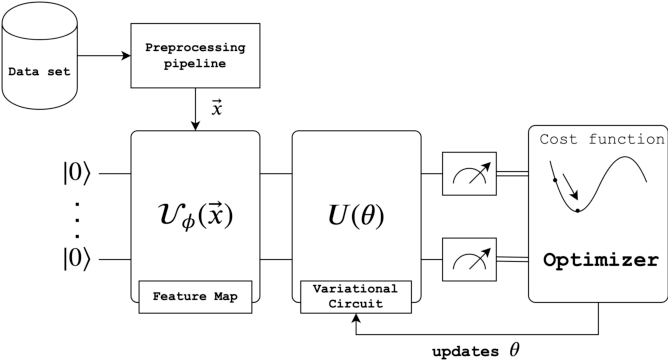
First, we will install the required dependencies needed to perform the task
!pip install --upgrade seaborn
!pip install --upgrade scikit-learn
!pip install --upgrade matplotlib
!pip install --upgrade pandas
!pip install --upgrade qiskit
import numpy as np
%matplotlib inline
import matplotlib.pyplot as plt
import seaborn as sns
import pandas as pd
from sklearn.decomposition import TruncatedSVD
from sklearn.manifold import TSNE
from qiskit import *
import numpy as np
from qiskit.aqua.utils import split_dataset_to_data_and_labels, map_label_to_class_name
from qiskit.aqua import QuantumInstance
from qiskit.aqua.algorithms import VQC
import time
You first have to download the training dataset from http://yann.lecun.com/exdb/mnist/ and save it in a .csv file format. We will give this file the name mnist_train.csv in the dataset folder. We will also download the testing dataset and save it as mnist_test.csv. You will have to have the python file in the same directory as the training and testing datasets to run the code. An image size of size 28 is initialized.
image_size = 28 # width and length are equal
data_path = "./dataset/"
train_data = np.loadtxt(data_path + "mnist_train.csv", delimiter=",")
test_data = np.loadtxt(data_path + "mnist_test.csv", delimiter=",")
The testing dataset has the same form except it has 10000 data points. In order to get an idea of a picture of a digit inside the dataset, we will run the following code.
image = train_data[:, 1:][1].reshape((image_size, image_size))
plt.imshow(img)
plt.show()
The dimension of the data corresponds to the number of qubits required in order to encode the data for the quantum feature maps we will later initialize. Since quantum computers today can only manipulate 50 qubits, we cannot work with large number of qubits like 784, therefore encoding data with dimension 784 is not viable.
Therefore, we will have to make use of the truncated Singular Value Decomposition (SVD) and t-distributed stochastic neighbor embedding (t-SNE) methods to reduce the dimension down to 10 and then to 2. If you're interested in learning about dimensionality reduction for the MNIST dataset you can read Colah's blog.
We will first truncate the dataset to 10000 data points so that it becomes easier to apply the TruncatedSVD and TSNE techniques.
#Extracting features and labels from the dataset and truncating the dataset to 10,000 datapoints
train_data_features = train_data[:10000, 1:]
train_data_labels = train_data[:10000, :1].reshape(10000,)

# Using SVD to reduce dimensions to 10
tsvd = TruncatedSVD(n_components=10)
X_SVD = tsvd.fit_transform(train_data_features)

# Use t-SNE technique to reduce dimensions to 2
np.random.seed(0)
tsne = TSNE(n_components=2)
train_data_features_reduced = tsne.fit_transform(X_SVD)
We will plot out the dataset to see if there is some sort of clustering due to classification of digits in the reduced dataset. We will need to create a pandas dataframe and using seaborn to plot the data.
# function to help plot the 2-D dataset
def plotdataset(X, Y, c1, c2, N):
    lbl1 = f'Component {c1}'
    lbl2 = f'Component {c2}'
    df = pd.DataFrame({lbl1:X[:N,c1], lbl2:X[:N,c2], 'label':Y[:N]})
    sns.lmplot(data=df, x=lbl1, y=lbl2, fit_reg=False, hue='label', scatter_kws={'alpha':0.5})
plotdataset(train_data_features_reduced, train_data_labels, 0, 1, N=2000)
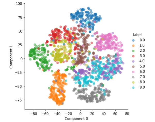
0 and 1 are well separated on opposite corners as they are easily distinguishable, however, 4 and 9 are overlapping as corresponding to purple and blue data points.
We will extract data points corresponding to the digits 0 and 1 from the reduced dataset and normalize their features to be between 0 and 2.
We need to normalize the data because the values will be inserted into a quantum feature map.
zero_datapoints_array = [] #an array of the data points containing value 0
one_datapoints_array = []# an array of the data points containing value 1
for i in range(10000):
    if train_data_labels[i] == 0:                   # extracting zeros
        zero_datapoints_array.append(train_data_features_reduced[i])

for i in range(10000):
    if train_data_labels[i] == 1:                   # extracting ones
        one_datapoints_array.append(train_data_features_reduced[i])

zero_datapoints_array = np.array(zero_datapoints_array)
one_datapoints_array = np.array(one_datapoints_array)

def normalize(arr, max_val, n):
    a = np.divide(arr, max_val)
    return a + n

zero_datapoints_normalized = normalize(zero_datapoints_array, 100, 1)
one_datapoints_normalized = normalize(one_datapoints_array, 100, 1)
We will follow the Variational Quantum Classifier (VQC) method as proposed in the paper Havlicek et.al to classify the digits using the concepts of quantum mechanics.
Similar to classical supervised machine learning algorithms, the VQC has a training stage (where data points with labels are provided and learning takes place) and a testing stage (where new data points without labels are provided which are then classified).
The main steps of this algorithm are:
1. Load Data onto the Quantum Computer by Applying a Quantum Feature Map Φ(x)
2. Build and apply short-depth Variational Circuit W(θ).
The Quantum Feature Map of depth d is implemented by the following circuit.
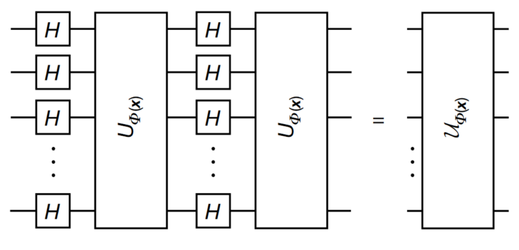
We will first learn how to configure inbuilt quantum feature maps in Qiskit Terra (Circuit Library) and then how to build a custom feature map. A feature map is a variational circuit.
Some of the feature maps include:
Let us first import the required libraries. We will test out the PauliFeatureMap first with
paulis=['Z', 'Y', 'ZZ'].
from qiskit.circuit.library import ZZFeatureMap, ZFeatureMap, PauliFeatureMap
feature_dim = 2
pauli_feature_map = PauliFeatureMap(feature_dimension=feature_dim, reps=1, paulis = ['Z','X','ZY'])
pauli_feature_map.draw()
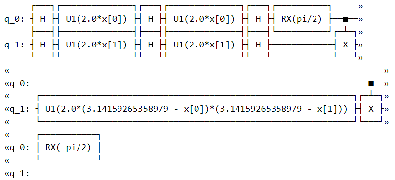
These are the feature maps present in Qiskit. However, these feature maps may not perform well on all datasets. For a particular dataset, finding a quantum feature map that can spread the data points in Hilbert space in such a way that a hyperplane can be drawn to classify them is important to gain higher accuracies for our model(this is the basics of support vector machines).
We also want that the corresponding quantum feature map circuit is shallow( have a small circuit depth) as this reduces quantum decoherence, leading to higher accuracies. If you are interested in learning about errors, decoherence and error mitigation techniques, you can look at this section of the Qiskit textbook.
Generally, we want to construct custom feature maps for increasing the accuracy of classification.
In this step we will append a variational circuit to the feature map. The parameters of this variational circuit are trained using classical optimizers until it classifies the data points correctly. This is the training stage of the algorithm and accuracy of the model depends on the variational circuit one chooses.
Constructing using Real Amplitudes:
Let us create a variational circuit using the inbuilt Real Amplitudes method. Check out the documentation page to understand how Real Amplitudes work.
from qiskit.circuit.library import RealAmplitudes

num_qubits = 2

variational_circ = RealAmplitudes(num_qubits, entanglement='full', reps=3)
We can also use the EfficentSU2 method to create the variational circuit.
var_circuit = EfficientSU2(feature_dim, reps=2)
The following steps need to be done in order to create a custom feature map:
from qiskit.circuit import QuantumCircuit, ParameterVector

num_qubits = 3
iter = 1              # number of times you'd want to repeat the circuit

x = ParameterVector('x', length=num_qubits)  # creating a list of Parameters
custom_circ = QuantumCircuit(num_qubits)

# defining our parametric form
for _ in range(iter):
    for i in range(num_qubits):
        custom_circ.rx(x[i], i)
    for i in range(num_qubits):
        for j in range(i + 1, num_qubits):
            custom_circ.cx(i, j)
            custom_circ.u1(x[i] * x[j], j)
            custom_circ.cx(i, j)

custom_circ.draw()
"How" a custom feature map is created is still not clear and in research.
Let's apply the VQC method in Qiskit Aqua to solve the task of classifying digits 0 and 1. We will take a very small subset of 20 training datapoints and 10 testing datapoints. We also keep 5 points per label as a validation set. We will first define the training and testing inputs based on the dataset we initialized before.
train_size = 20
test_size = 10
dp_size_zero = 5
dp_size_one = 5

zero_train = zero_datapoints_normalized[:train_size]
one_train = one_datapoints_normalized[:train_size]

zero_test = zero_datapoints_normalized[train_size + 1:train_size + test_size + 1]
one_test = one_datapoints_normalized[train_size + 1:train_size + test_size + 1]

training_input = {'A':zero_train, 'B':one_train}
test_input = {'A':zero_test, 'B':one_test}

# datapoints is our validation set
datapoints = []
dp_zero = zero_datapoints_normalized[train_size + test_size + 2:train_size + test_size + 2 + dp_size_zero]
dp_one = one_datapoints_normalized[train_size + test_size + 2:train_size + test_size + 2 + dp_size_one]
datapoints.append(np.concatenate((dp_zero, dp_one)))
dp_y = np.array([0, 0, 0, 0, 0, 1, 1, 1, 1, 1])
datapoints.append(dp_y)

class_to_label = {'A': 0, 'B': 1}
We have not used a custom feature map in this implementation, however the custom feature map we defined before will still work and you can try out different combinations of parameters to see which feature map gives highest accuracy.
seed = 10598
feature_dim = zero_train.shape[1]

feature_map = ZZFeatureMap(feature_dimension=feature_dim, reps=2, entanglement='linear')
feature_map.draw()
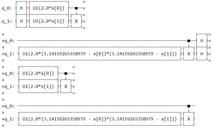
A classical optimization routine changes the values of our variational circuit and repeats the whole process again. This is the classical loop that trains our parameters until the cost function value decreases. You can look at the code and the optimization step as given in the Qiskit Textbook to understand the classical optimization process.
VQC Aqua provides a few classical optimizer methods:
We will use the COBYLA optimizer method
from qiskit.aqua.components.optimizers import COBYLA

cobyla = COBYLA(maxiter=500, tol=0.001)
from qiskit.circuit.library import EfficientSU2, RealAmplitudes

var_circuit = EfficientSU2(feature_dim, reps=2)
This is what our final circuit will look like.

# initilizing backend
backend = BasicAer.get_backend('qasm_simulator')
backend_options = {"method": "statevector"}

# creating a quantum instance
quantum_instance = QuantumInstance(backend, shots=1024, seed_simulator=seed, seed_transpiler=seed, backend_options=backend_options)

#initilizing VQC object
vqc = VQC(optimizer=cobyla, feature_map=feature_map, var_form=var, callback=call_back_vqc, training_dataset=training_input,
         test_dataset=test_input, datapoints=datapoints[0])
result = vqc.run(quantum_instance)

print("testing accuracy: {}".format(result['testing_accuracy']))
print("prediction of datapoints:")
print("Actual: {}".format(map_label_to_class_name(datapoints[1], vqc.label_to_class)))
print("prediction:   {}".format(result['predicted_classes']))
If you run this, then the testing accuracy output is 1.0. This means that our Variational Quantum Circuit is 100% accurate. We can check this by printing the actual and predicted values and we see that wherever there is a 0 in the actual dataset, we have predicted a 0 and vice-versa.
About
Support
Every week, our team curates the most important news, events, and opportunities in the quantum space. Our subscribers gain early access to opportunities and exclusive interviews with prominent individuals. You don't want to miss out.